Phoenix vs ClickHouse: Why the Fight Never Ends

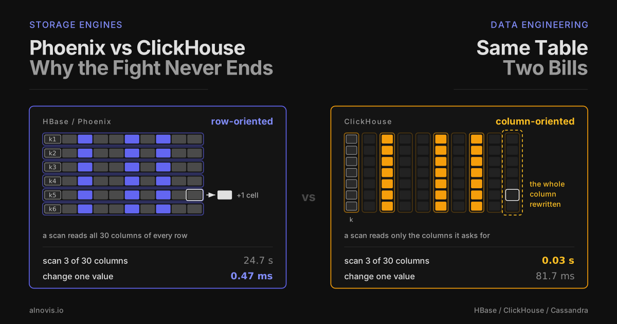
The Fight

The system I work on keeps its sales documents in two databases, and every few weeks the same argument comes back to our standup.

One side: "The data is already in Phoenix. Let's build the monthly report there, why copy anything?" The report is a GROUP BY over a few months of documents. It runs for minutes, the region servers sweat, and the dashboard gives up first.

The other side: "It's one document with the wrong status. Just fix it in ClickHouse." The fix is an ALTER TABLE ... UPDATE. It changes one row and rewrites far more than one row, and a day of such fixes leaves a queue of mutations behind it.

I have argued both sides. Sometimes in the same week.

The usual way to settle it is a label. Phoenix is OLTP, ClickHouse is OLAP; one stores rows, the other stores columns; one is an LSM tree, the other is not. The labels are not exactly wrong, but none of them says what a given query will cost, so the argument comes back.

This post takes both engines apart down to what they read and write, on a test stand that holds the same ten million documents in each. Underneath there are four knobs. Each one comes with a small formula, and the formula says in advance which side of the standup is going to lose.

The first surprise comes before any formula: Phoenix is not even in the ring.

Phoenix Is Not in the Ring

Phoenix is a SQL layer over HBase. It stores nothing of its own: it compiles SQL into the operations HBase already has.

• A table becomes an HBase table. The primary key columns are concatenated into the row key; every other column becomes a cell in a column family, under a short encoded qualifier (two bytes by default) instead of the column name.
• A SELECT by the full primary key becomes a lookup of one row key. A range or a full SELECT becomes scans, at least one per region, which the client runs in parallel.
• A GROUP BY runs in two steps: region servers compute partial aggregates in coprocessors, next to the data, and the client merges them.
• A secondary index is another HBase table, and every upsert writes to it as well.

Summing next to the data is Phoenix's main trick: only partial sums cross the network, not rows. It can add work too, an index write for every upsert. What it cannot change is what a region server reads from disk to answer. That is HBase, block by block.

So the fight is named after Phoenix, but the physics is HBase against ClickHouse's MergeTree. Billing Phoenix's overhead to HBase, or crediting HBase's physics to Phoenix, would make every comparison lie. From here on the stand talks to HBase directly, through its native client (Get, Put, Scan), and Phoenix comes back only where it adds or removes a cost.

Both Are Log-Structured

The textbook frame says that an OLTP store is a B-tree that updates its pages in place, and an OLAP store is something else entirely. Neither engine here updates anything in place. Their write paths have the same shape:

An HBase Put goes to the write-ahead log and into the memstore, a sorted buffer in memory; at 128 MB the memstore is flushed into an HFile, and compactions later merge HFiles into bigger ones. A ClickHouse INSERT block is sorted in memory and written as a new part, a directory of column files; background merges later combine parts into bigger ones.

Buffer, immutable sorted file, merge later. Both are log-structured merge designs. "LSM vs B-tree" is not this fight.

Same shape, same failure. The first load on the stand wrote ten million rows into HBase in key order, so at any moment every write went to the one region whose range was being filled. Flushes produced files faster than compaction merged them. At 17 files in the region, one over hbase.hstore.blockingStoreFiles, HBase began delaying each flush by up to 90 seconds. The memstore kept growing to its blocking size, flush size times the block multiplier, 128 MB x 4 = 512 MB, and then the region refused writes:

RegionTooBusyException: Over memstore limit=512.0 M

until a compaction caught up. ClickHouse has the same failure under another name. When inserts create parts faster than merges combine them, it first slows inserts down (parts_to_delay_insert) and then rejects them with "Too many parts" (parts_to_throw_insert). One write stall, two names.

Cassandra, the third engine on the stand, belongs to the same family: commit log and memtable, flushed into SSTables, merged by compaction, the write path of Google's Bigtable that HBase copied as well. Its storage choices sit close to HBase's, so it gets no separate pass through the first three knobs. It parts ways on the fourth, who owns a key, and that is where it comes back.

Four Knobs

If both engines append and merge, what makes one of them good at the monthly report and the other at fixing one document? Four choices, each a dial that every log-structured engine has to set somewhere:

knob	HBase	ClickHouse	Cassandra
1. rows behind one index entry	a block: 64 KB of whole rows	a granule: up to 8,192 rows	two levels: every partition, then 64 KB inside one
2. what one unit of read holds	whole rows, every column of the family	one column, compressed	like HBase: whole rows
3. what a change rewrites	nothing now: a new cell version, merged later	the changed columns of every part with a matching row	like HBase
4. who owns a key on many nodes	one server per key range, storage shared	the shard the sharding key picks, own disks	a hash ring, any node coordinates

Every setting is cheap on one side and expensive on another. The sides have a name, the RUM triangle: the cost of Reading, of Updating, and of the Memory or space the data takes. The next four sections measure what each knob costs, and the triangle at the end puts them together.

Knob 1: How Many Rows Stand Behind an Index Entry

Neither engine indexes every row. Both keep a sparse index: the rows are sorted by key and cut into chunks, and the index remembers where each chunk starts. To find one row, the engine finds its chunk and reads the chunk whole.

How big the chunk is, is the first knob. Call it g, the rows behind one index entry:

ClickHouse sets g = 8,192 rows and calls the chunk a granule. The stand's table has 10 million rows and a primary index of 1,224 marks: 4.9 KB, always in memory (marks and primary_key_bytes_in_memory in system.parts). A billion rows would need about 122 thousand marks, still nothing. The price sits on the other side of the formula: to return one row, ClickHouse processes its whole granule, 8,192 rows of every column the query asks for.

HBase cuts by bytes, not by rows. A block closes at 64 KB of uncompressed cells, which for these 1.2 KB rows is about 58 rows. Its g is 140 times smaller, so its index is 140 times bigger: 172,472 entries for the same table, one per data block (the blocks a full scan counts in HBase's server-side scan metrics). That no longer fits in memory as one array. It is stored in blocks itself, next to a bloom filter per file that answers "is this key in this file at all".

One point read of a whole row, caches warm, median of 2,000 random keys:

	g	index	to return one row	median
ClickHouse	8,192 rows	1,224 marks, 4.9 KB	one granule processed, 8,192 rows	3.47 ms
HBase	~58 rows	172,472 entries	one 64 KB data block accessed, plus 256 KB of bloom and index blocks, all in the block cache	0.15 ms

"One granule" counts rows, not bytes, and the disk sees something else. A separate run with ClickHouse's own counters, per point read:

ClickHouse, one row	processed	decompressed	compressed bytes read (page cache)
whole row, 30 columns	1.70 MB	2.82 MB in 38 blocks	525 KB
3 columns	180 KB	328 KB in 5 blocks	90 KB

More is decompressed than processed because a compressed block holds at least 64 KB. A one-byte column such as status takes 8 KB per granule, so one of its blocks covers eight granules, and reading one granule means decompressing all eight. The three-column read is five blocks of exactly 64 KB: the three columns and the two key columns the filter needs. (The volumes come from that separate run, the latency from the timed one.)

A SELECT 1 through the same HTTP client takes 0.6 ms: the baseline of any query on this stand, parsing, planning and the round trip included. Above that baseline, three columns cost 0.8 ms and all thirty cost 2.9 ms. That is the part that grows with the columns asked for; decoding the granule is in it, and so is opening one column file per column. The timing alone does not split the two.

HBase pays for its small g in a way the formula hides. Of the ~320 KB a Get touches, 64 KB is the data block; the rest is one 128 KB chunk of the bloom filter and one leaf block of the index, up to 128 KB. All of it comes from the block cache here, so it costs microseconds, but it is three blocks per Get, not one. The card in the next section counts data blocks only, and for one file per region it says one; the index and the filter are the reads it leaves out.

This is the first standup scene in reverse. For a single row ClickHouse is 24 times slower, and not because it is badly built: it chose a g that makes its index free, and a point read pays for that choice.

Cassandra Lets the Schema Choose g

Cassandra's index has two levels. The partition index has an entry for every partition; a sample of it, one entry in 128, sits in memory, next to a bloom filter on the partition key. Inside a partition the rows are sorted by the clustering key, and a partition bigger than 64 KB gets an index of its own, an entry per 64 KB.

So in Cassandra g is a schema decision, and the stand can turn it like a dial. The same ten million rows went in twice: once with a partition per register, a thousand documents ordered by number inside it, and once with a partition per document. Three nodes, everything summed:

partition per	partitions	index on disk	bloom filter	space	point read
register	10,000	1.45 MB	12.6 KB	684 MiB	223-231 µs
document	10,045,874	257 MB	12.6 MB	1,564 MiB	206-216 µs

The card holds in a third engine. A thousand times the entries cost a thousand times the bloom filter (ten bits per partition in both tables) and 177 times the index on disk. The point read got 15 microseconds faster, and the table more than doubled. Of the extra 880 MiB, 245 MiB is index; the rest is most likely the price of the order. With a partition per document the rows lie in hash order, so the rows of one register, whose constant columns compress well side by side, are scattered across the file. That part is a reading, not a measurement.

What the small partitions did buy is the bloom filter:

With a partition per register, every file holds a slice of every register, and the filter lets every file through. With a partition per document, each document lives in exactly one file, and the read traces show the filter skipping 4.3 files per read. "Exactly one" holds for this table, loaded once and never updated: an update writes a newer piece of the partition into a newer file, and from then on the filter lets two through. That is the p (h - 1) term of the next section's card at work: a filter only helps when its key is as fine as the read.

Knob 2: What One Read Brings Back

The second knob is what sits inside the chunk. An HBase block holds sorted cells: all the cells of about 58 rows, every column of the column family, one row after another. A ClickHouse granule is not one chunk but one per column, each compressed on its own. A query that needs three columns opens three files and never touches the other twenty-seven.

For a scan that is the whole story, and it fits a formula. For a point read the same layout works the other way round:

ClickHouse read 100 MB for the narrow scan: status 10 MB, payment_type 10 MB, amount 80 MB, uncompressed by its own counter. That is B_col to the byte. Compressed, it read 52.6 MB, all from the page cache on this stand: the three column files and nothing else. The wide scan read 315 MB compressed, the whole table. HBase read 172,472 blocks for the narrow scan and the same 172,472 for the wide one, 11.3 GB from the file system either way on the uncompressed table. Asking HBase for 3 columns did not change what it read. It changed what crossed the network.

The k is not a rounding error. In the uncompressed HBase table about 80% of the bytes are keys: every cell carries its row key, family, qualifier and timestamp, about 36 bytes (inferred from the table's size, not read out of an HFile), next to 8 bytes of value on average. Prefix encoding and LZ4 bring the table from 11,180 MiB down to 792 MiB. ClickHouse keeps the same rows in 299 MiB.

And the point read flips the result. Both tables compressed, medians:

The same numbers as a table

	HBase (FAST_DIFF + LZ4)	ClickHouse (LZ4 + delta codecs)
scan, 3 of 30 columns	24.7 s	0.03 s
scan, all 30 columns	26.9 s	0.35 s
point read, whole row	170 µs	3.47 ms
point read, 3 columns	197 µs	1.44 ms
on disk	792 MiB	299 MiB

Each point marks one term of the card. ClickHouse's whole row costs 2.4 times its three columns: one block per column asked for, the |Q| term. HBase's whole row costs about the same as three columns: the block holds the row either way, and fewer columns only save serialization.

Two caveats, both against HBase. Its LZ4 runs in Java on this stand (the native Hadoop libraries are not loaded), and the aggregation runs in the bench client. Neither explains the gap: the wide scan moves nine times more cells to the client than the narrow one and takes only 1.1 times longer. The time is in the blocks. Phoenix's coprocessors would save the transfer, not the blocks.

HBase has one knob toward columns of its own: column families are stored apart, so putting the few hot columns into a family of their own is a column store by hand. It works for the columns you knew about in advance.

Knob 3: What a Change Rewrites

Now the second standup scene: one document with the wrong status. Both engines keep their files immutable, so neither of them can change a value in place. The only question is what each of them writes instead, and when.

An HBase Put writes one new cell with a newer timestamp and leaves the old one where it is. A read merges the memstore with the files and the newest timestamp wins. The old cell stays on disk until a compaction merges its file with a newer one. A minor compaction merges a selection of files; a major compaction rewrites every file of a column family's store, whatever changed. The stand's table has one column family, so a major compaction there rewrites every cell of the region.

A ClickHouse ALTER TABLE ... UPDATE is a mutation: it finds the rows, then writes a new version of every part that has one.

P is the set of parts the mutation has to check; on a real table the partition key and the primary index can rule many of them out. On the stand the table is one part of 10 million rows, so there is nothing to rule out: P and T are the same single part, W is the key (register_id, doc_id) and S is status. One update read 130 MB, register_id 40 MB plus doc_id 80 MB plus status 10 MB, uncompressed, exactly the card. It wrote the status column of the part, 1.39 MB compressed, to change one byte.

The card also says the cost is set by the touched parts and columns, not by the number of rows changed. On this stand, updating more rows in the same part barely changes the cost:

rows changed at once	1	1,003	100,000
ClickHouse ALTER UPDATE, wait for the mutation	157 ms	139 ms	138 ms
HBase Puts, one batch	(warm-up)	310 ms	850 ms

(The 1-row HBase batch measured the client's first region lookup, not the Put.)

So the scene at the standup is a stream of single fixes, and there the gap is widest. A hundred single-row updates, one after another, medians: an HBase Put 472 µs, a ClickHouse mutation 81.7 ms. That is 173 times: 0.05 s of work for HBase, 8 s for ClickHouse, for the same hundred statuses.

ClickHouse Can Update, by Not Updating

Both sides of the standup already know the way out: do not change the value, append a new version and let reads pick the newest. HBase does that natively. ClickHouse has done it for years with ReplacingMergeTree and argMax, which is the trick an earlier post is built on. And ClickHouse 26.3 does it inside the engine, as a beta: a lightweight UPDATE writes a small patch part with only the changed rows, readers apply the patches on the fly, and a merge or APPLY PATCHES folds them into the data later.

The same hundred single-row updates as a lightweight UPDATE: 3.12 ms each, 26 times faster than the mutation and still 6.6 times slower than HBase. The bill did not disappear, it moved:

The reader's share is not small for its size. With one patch part pending, a part of 100 rows and 1,900 bytes, the narrow scan read 180 MB instead of 100 and took twice as long. On this stand the pending patch added roughly 8 bytes per scanned row, though only 100 of the 10 million rows had changed. APPLY PATCHES rewrote the status column once, in 103 ms, and the scans went back to 100 MB. (Measured on one part with one patch part, which the background merge had already made out of the hundred; many unmerged patches were not measured.)

"ClickHouse cannot update" turns out to be wrong. It can, by doing what HBase does: write a small delta now, merge it on every read, fold it into the data later. A change can impose costs at three points: when it is written, while it is read, and when the data is rewritten later. Each engine, and each way of updating inside one engine, chooses a different distribution; a plain ALTER UPDATE pays everything at the first. Cassandra writes a new cell like HBase, and its later rewrite, the compaction strategy, is a knob of its own, the one the triangle at the end turns.

Knob 4: Who Owns a Key When There Are Many Nodes

Everything so far happened on one server. Big data rarely does, and the fourth knob is the one that only exists on many nodes: what the unit of placement is, and who moves it. The three engines give three different answers.

Before the numbers, an honest limit of the stand. All the pods run on one machine with six physical cores, so a second node adds a CPU quota, not hardware. Each half of the wide scan, alone on its shard, took 176 ms; both halves at once took 340 ms each. Speedup cannot be measured here. What can be measured is where the work goes and how many nodes a request has to touch, and that is what this section is about.

One Read, One Node, or a Detour

HBase has no coordinator at all. The client reads the region locations once from the hbase:meta table, caches them, and sends every Get straight to the server that owns the key. With two region servers both answered a whole-row Get in about 250 µs, and no second query existed anywhere.

ClickHouse puts an initiator in front of the shards: the server that receives the query plans it again, sends it to each shard over TCP and merges what comes back. For one row that detour cost more than the read itself:

The owning shard did exactly the work a single server does, a granule in 4 ms. The initiator added 4 to 5 ms of its own on top, a fixed cost per query that is invisible under a 0.3 s scan and doubles a point read. Without the sharding key in the WHERE, it also sent the query to the shard that does not have the row, and that shard read a granule of its own to find nothing: 17.3 thousand rows processed per lookup instead of 8.2. With optimize_skip_unused_shards the query goes to the owner only. That halves the cluster's work but saves just 0.5 ms of latency, because the two shards were asked in parallel.

Cassandra makes the detour a choice of the client. Every node can coordinate. A token-aware driver computes the partition's token from the bound key and sends the request to a replica, like the HBase client. Send it anywhere else, and that node forwards it, like a ClickHouse initiator. One table, both paths, measured inside the same run: 245 µs when the coordinator was the replica, 363 µs when it forwarded. On this read at ONE, the extra coordination cost was about 120 µs, largely consistent with one more network hop. A coordinator also enforces the consistency level and collects and reconciles the answers; at ONE there is little of that to do.

Where New Rows Go

Ownership by key range has a famous weakness: a key that only grows. Two million new documents written in doc_id order into an HBase table with eight regions on two servers:

With the plain key, every new row went to the last region and so to one server, while the other server and seven of the eight regions sat idle. Pre-splitting the existing key range does not help: the new writes still land beyond the last split point. Salting, what Phoenix calls SALT_BUCKETS, spread the same rows exactly evenly and wrote 1.5 times faster from the same client. Its price is on the read side: a range of new documents is now eight scans instead of one. On an idle cluster the eight parallel scans even won, 4.1 ms against 11.3. On a loaded one they are eight times the requests; that was not measured.

With a hash-based sharding expression, ClickHouse makes the same trade; the expression is the user's, and it need not hash at all. Cassandra's partitioner makes it by default. A hash spreads monotonic keys by itself, and in exchange a range that is not inside one shard or partition goes to every node. Cassandra goes further: there is no order across partitions at all, only inside one.

What Moving Costs

When ownership changes, the knob decides whether bytes move. On the stand, in HBase:

HBase, two region servers	took	readers saw	bytes rewritten
move a region to the other server	1.0 s	one refused Get, retried in 138 ms	none: the new owner opens the same files
split a 99 MiB region	1.1 s	one pause of 757 ms	none at once: both daughters start as references to the parent's file, and rewrite their halves in a compaction within a minute
merge the daughters back	0.6 s		none at once, references again

Ownership in HBase is metadata, because the storage is shared; the bytes follow later, at compaction's pace. It is the deferred bill of knob 3, now for knob 4. A ClickHouse shard owns its rows on its own disks, so there is nothing to hand over: moving rows means copying them, and a new shard only changes where new rows go. In Cassandra a new node takes over a slice of the ring and streams its data from the others, about 1 / (S + 1) of it; that was not measured here. Its placement did need no pre-split at all: with 16 virtual nodes per server, the three nodes got 35.7, 32.7 and 31.6% of the rows on their own.

The Coordinator's Bill Grows With Groups

A scan's partial results have to meet somewhere, and for a GROUP BY that is the initiator. Its work grows with the number of groups, not with the number of rows. Ten million rows on two shards:

10M groups		wall	initiator CPU	initiator receives
GROUP BY doc_id	one server	261 ms
	two shards, initiator merges	896 ms	1,360 ms	92 MB of partial states
	two shards, told no group crosses shards	229 ms	5 ms	almost nothing
GROUP BY register_id, doc_id	two shards, initiator merges	1,017 ms	2,041 ms	124 MB
	two shards, sharding key recognised	293 ms	6 ms	almost nothing

With ten million groups the initiator received every shard's partial states and spent as much CPU merging them as one server needs for the whole query. The two-shard cluster was 3.4 times slower than one server. When ClickHouse may treat the groups as disjoint, the initiator does nothing. You can tell it so (distributed_group_by_no_merge = 2, correct here only because each doc_id lives on one shard), or it can work that out itself when the sharding key is in the GROUP BY. On 26.3 the second needed both optimize_distributed_group_by_sharding_key and optimize_skip_unused_shards; the first alone did nothing. For about a million groups the bill was mild: 132 ms of initiator CPU, 113 ms against 75 on one server. The sharding key, chosen once for writes, decides the read side too.

Replicas, and What "Acknowledged" Means

Only Cassandra in this post keeps replicas of its own: HBase leaves them to HDFS, and the ClickHouse cluster here had none. With three replicas, every request picks how many of them must answer. A point read, token-aware, warm medians:

consistency level	replicas that answer	median
ONE	1	264-280 µs
QUORUM	2	362-385 µs
ALL	3	400-439 µs

The coordinator asks the replicas in parallel; what changes with the level is how many answers it waits for. QUORUM waits for two replica responses instead of one, and on this stand that added roughly 100 µs, comparable to the forwarding penalty measured above. ALL waits for the slower of the two remote replicas as well.

The write side showed something no read did. The ten million rows were loaded at the driver's default, LOCAL_ONE: a write is acknowledged when one replica has it. Under that load the replicas reported 116 thousand dropped mutations, timing out on six shared cores, and the client saw no error. Hinted handoff did the catching up: after the load had ended, the hint dispatchers on all three nodes kept completing tasks, the replicas' local write counts kept rising, by 565 thousand in half an hour, and then no node had a pending hint left. The counters do not match one to one, and the number of hints written was not read: a hint is stored for a missing answer, not for a missing write, so the replayed writes, 1.8 million over the 30 million expected, include writes that had landed already. After compaction the three copies were exactly the same size, 717,670,958 bytes each; their contents were not compared. "Acknowledged" had meant one replica; the other two caught up in the background, without a repair.

The Triangle

In 2016 Athanassoulis and co-authors put a name to what every section above kept running into: the RUM conjecture. An access method can keep low any two of three overheads, the cost of Reading, of Updating and of the Memory or space the data takes, but not all three. Each knob is a way to move cost from one corner to another:

• Knob 1, a bigger g: the index shrinks (M), and every point read processes more rows (R).
• Knob 2, a column per unit of read: a scan reads only its columns and they compress well (R for scans, M), while a point read opens a block per column (R for point reads). Rows trade the other way.
• Knob 3, append a version instead of rewriting: cheap now (U), paid by readers who merge (R) and by old versions that take space (M) until the next rewrite.
• Knob 4 is not on the triangle. It multiplies whatever the other three cost by the number of nodes a request has to touch.

Both engines claim the R corner, each for its own kind of read: HBase for a point read, ClickHouse for a scan. That is the standup fight drawn as geometry. The positions are not coordinates measured on a common scale: each engine optimizes a different kind of read, and the RUM conjecture itself is about access methods, not whole databases. The picture shows directions, not distances. You can slide along the triangle, not out of it. Phoenix is not a point on it at all: a layer moves work between the client and the servers, not between the corners.

Cassandra Makes the Slide a Setting

In HBase and ClickHouse the position is built into the engine. In Cassandra one part of it is a table option: the compaction strategy decides how often data is rewritten (U) against how many files a read has to open (R). Cassandra 5.0 folds the classic strategies into one, the Unified Compaction Strategy, with a single parameter that slides from tiered (T4) through N to leveled (L10).

The stand wrote the same stream into four tables that differ only in that option: ten million rows, then five million updates of two columns at random rows. Then it waited until compaction had nothing left to do:

The same numbers as a table

strategy	rewrites per byte	SSTables opened per read	space over the floor	point read, median
STCS, the table default	3.75	3.27	+4.9%	293-329 µs
UCS T4	2.84	2.92	+3.5%	355-398 µs
UCS N	5.54	3.65	+5.0%	272-297 µs
UCS L10	8.49	1.66	+1.3%	237-251 µs
any, after a major compaction		1.00	0	223-299 µs

"Rewrites per byte" is what compaction wrote, divided by the size of the same table after a major compaction; the flush writes everything once more on top. SSTables per read are counted from read traces, one event per file a read opens.

From T4 to L10 the rewrites triple and the files a read opens halve. Settled, L10 reads as fast as a fully compacted table. That much is the textbook trade, measured.

The middle is not. N rewrote twice as much as T4 and still left reads opening the most files. A reading, from UCS's design rather than from its source: with flushes of a few megabytes and about 260 MB per node, a node holds some 65 flushes of data. That is about three levels at a fanout of 4, six at a fanout of 2 (N), two at a fanout of 10, and each level is a rewrite. On this workload, N was not a midpoint between T4 and L10. The default STCS was also behind T4 on both axes in this run. One stream and one stopping point, though: which levels happen to be full when the stream ends can move the count per read by a whole file.

Latency tells a different story from the file count. N opened the most files and still answered faster than T4: 272-297 µs against 355-398. L10, with the fewest files, was the fastest, so the count is not noise; but with every file in the page cache and the key cache warm, an extra file cost tens of microseconds at most, and something else, not traced here, outweighed it between N and T4. So the chart shows the trade between rewriting and files touched per read. The number of files is a useful measure of read cost and a poor predictor of latency on a warm cache; a cold disk would charge more per file.

Space barely moved: it stayed within 5% of the floor, because the updates touched two columns of thirty and the old versions were small. The bloom filter helped none of the strategies: with a partition per register every file holds a slice of every partition. The same rows with a partition per document read exactly one file of five or six without any help from compaction (knob 1 again). In Cassandra the schema moves the R corner as much as the compaction setting does.

Step back from the Cassandra numbers and they say what the whole post has been saying. A setting that makes one operation cheap does not make its cost go away. It moves the cost to another operation, or to a later moment. L10 rewrites more so that reads open fewer files; T4 rewrites less and reads pay for it. The UCS parameter is just the rare place where that move is a single word in a table definition.

So the standup question was never which database is better. Each engine moves the cost of an operation to another place and another time. HBase moves the cost of a write to a later compaction, and makes every scan read whole rows. ClickHouse pays for a change at once, by rewriting a column, or hands it to readers when the update is lightweight. Cassandra lets each table choose how much to rewrite and how many files to read. The fight starts when a workload's biggest cost lands where its engine put the bill.

So Which One

Back to the standup. Both scenes from the beginning, with the knob that decides each of them and what it cost on the stand:

Neither engine was wrong in either scene. Each scene was a workload whose dominant term belongs to the other engine's knob. The report is one scan over a few columns, and HBase reads whole rows. The fix is one value in one part, and ClickHouse rewrites the column. Both engines did exactly what their knobs say, and lost by factors of about 800 and 170.

So the choice can come from the knobs rather than from taste:

• Point reads against scans, and how many columns a query touches, decide knobs 1 and 2. A workload of point reads by key wants a small g and whole rows. A workload of scans over a few of many columns wants a granule and a file per column.
• How often rows change, and how scattered the changes are, decide knob 3. A stream of single-row fixes is a stream of column rewrites for a mutation, a few microseconds of WAL for HBase, and something in between for a lightweight UPDATE whose bill goes to the readers.
• The key decides knob 4. Route by it and a point read touches one node. Group by it and the coordinator has nothing to merge. Make it grow monotonically under a range partitioning, and one server takes every write.
• The SQL layer is a separate decision. Phoenix on HBase buys SQL, secondary indexes and partial aggregation on the region servers. It does not buy a different storage.

And when a workload honestly has both, a hot table of documents that change and a cold history that is scanned, the answer is two systems and a pipe between them, change data capture from one into the other, with its own cost in lag and operations. Or one engine and the append-a-version trick, which is what the cells in the earlier post do inside ClickHouse. Either way the cost of the other corner does not disappear. It gets a place and a time you chose.

None of this will end the argument at our standup. It comes back every few weeks, as it always has. But the next time someone says "the data is already in Phoenix", there is a question to ask before anyone argues: which knob does this query's biggest term turn? I still argue both sides, sometimes in the same week. Now at least I know which side I am on before I start.

Every number in this post, and the stand they come from

One k3s node, an AMD Ryzen 5 5600X with 6 physical cores and 12 hardware threads, shared by every pod. ClickHouse 26.3.9.8, 5 CPU and 12 GiB per server. HBase 2.5.16, standalone with 5 CPU, 12 GiB and an 8 GiB heap, or two region servers with 5 CPU, 6 GiB and a 4 GiB heap each over one shared volume. Cassandra 5.0.9, three nodes with 4 CPU, 5 GiB and a 2 GiB heap each. One synthetic table of 10 million documents, 30 columns, the same rows in every engine. Latencies are medians of warm runs.

	HBase	ClickHouse	Cassandra
on disk, 10M rows	792 MiB (FAST_DIFF + LZ4)	299 MiB (LZ4 + delta codecs)	684 MiB (LZ4, a partition per register)
point read, whole row	170 µs; 250 µs on two servers	3.47 ms	216-243 µs, token-aware
point read, 3 columns	197 µs	1.44 ms
point read through a coordinator	none	8.3 ms (Distributed)	362-364 µs (forwarded)
scan, 3 of 30 columns	24.7 s	0.03 s
scan, all 30 columns	26.9 s	0.35 s
one single-row update	472 µs (Put)	81.7 ms (ALTER UPDATE), 3.12 ms (lightweight)
100,000 rows changed at once	850 ms	138 ms
GROUP BY of 10M groups, one node and two		261 ms and 896 ms
a region moved, split, merged	1.0 s, 1.1 s, 0.6 s
a monotonic key, rows per server	2,000,000 and 0; salted 1,000,000 each
read at QUORUM of 3 replicas			362-385 µs
compaction rewrites per byte, T4 to L10			2.84 to 8.49

Closing and Prior Art

None of the four knobs is new, and neither is the triangle. The log-structured merge tree is O'Neil, Cheng, Gawlick and O'Neil, "The Log-Structured Merge-Tree (LSM-Tree)", Acta Informatica, 1996. HBase and Cassandra both store data the way Google's "Bigtable: A Distributed Storage System for Structured Data" (Chang et al., OSDI 2006) describes, and Cassandra places it the way Amazon's "Dynamo" (DeCandia et al., SOSP 2007) does. The column store half of the story is in "C-Store: A Column-oriented DBMS" (Stonebraker et al., VLDB 2005) and in Abadi, Madden and Hachem, "Column-Stores vs. Row-Stores: How Different Are They Really?" (SIGMOD 2008). The triangle is "Designing Access Methods: The RUM Conjecture" (Athanassoulis et al., EDBT 2016). Chapter 3 of Martin Kleppmann's Designing Data-Intensive Applications tells the same story at book length.

What was ours is only the stand: the same ten million documents in three engines, the formula cards held against the engines' own counters, and an honest note every time a number did not fit. Several did not. A point read decompresses more than its granule. A pending patch taxes every row of a scan. Replicas left behind by writes acknowledged at LOCAL_ONE caught up by themselves, minutes later. And the middle setting of a compaction slider was not in the middle. Each of those taught more than the numbers that fit.

The standup argument will come back. It should. Behind it is a real workload with a real dominant cost, and the knobs say where that cost goes.